Priming Indices in ITensor

Thomas E. Baker—August 21, 2015

Each index of an ITensor is an object of type Index. Each Index represents some vector space over which the tensor is defined.

For example, a matrix product state (MPS) tensor has one physical Index of type Site. If the MPS is the wavefunction of a chain of S=1/2 spins, then a site index of a particular MPS tensor represents the physical "degrees of freedom" of that site. If the meaning of this site index ever changes (we give an example below), then we should replace the original Index with a different one. But what about indices that have the same meaning, but which we do not want the ITensor * operation to contract? (Recall that taking the * product of two ITensor contracts all pairs of matching indices.)

For example, consider the @@S_z@@ operator. This operator has two indices:

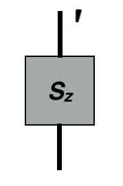
When acting @@S_z@@ onto a wavefunction, we only want one of the indices (the bottom one in the diagram) to be contracted, with the top one remaining uncontracted. Setting the prime level of the top index to 1 enforces this behavior, assuming the wavefunction has unprimed indices.

We will detail in this article how to use primes on indices and best practices.

When not to use Primes

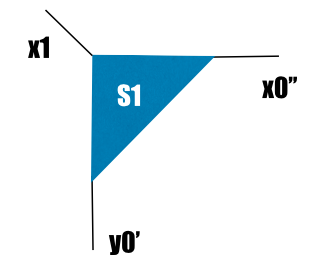
An example where we might want to introduce a new Index, rather than priming an existing one, is when coarse graining a lattice (in some real-space RG procedure). If we go from a fine lattice to a coarser one, then we have a diagram that looks like the diagram on the left:

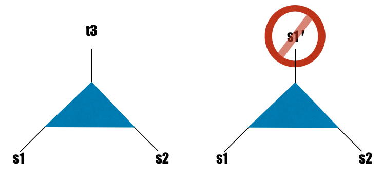
The local physics has changed on the coarser level. A single site now corresponds to two sites of the original lattice and could have a dimension ranging from 1 to the square of the original lattice dimension. If the new coarse-grained lattice happens to have the same local dimension as the old, it might be tempting to "recycle" the index s1 by using a primed copy of it as the new site index (as in the diagram on the right). But in light of the new physics, we should just introduce a new Index (left) instead of using a primed version of an existing Index (right).

Functions that Prime Indices

In the following, we use "ITensor" to refer to either ITensors or IQTensors, since they have the nearly same interface. For an exhaustive list of all class methods and functions for manipulating prime levels, see the documentation for ITensor objects.

Let us look at some of the most common functions used to manipulate ITensor prime levels. These functions all return an copy of the ITensor with modified prime levels. (ITensors are inexpensive to copy, and only copy their data when absolutely needed.)

Some priming functions act on all the indices:

• prime(ITensor) - Return a copy of the ITensor with all index prime levels incremented by one
• prime(ITensor,int) - Increment the prime level of each index by "int" (can also be negative)

You can also just raise the prime level of indices of a given IndexType

• prime(ITensor,IndexType) - Increment all indices of IndexType Type

For example, prime(psi,Site) raises the prime level of all indices of type Site.
Indices can be given custom IndexTypes such as Link, Site, etc.

• prime(ITensor,Index,int) - Changes the prime level of the specific index "Index" on an ITensor by value "int"
• prime(ITensor,Type,int) - Increment the prime level of all indices having type "Type" by "int".

To reset all prime levels back to zero, use:

• noprime(ITensor) - sets prime level of an ITensor to zero

Sometimes it is convenient to refer to indices by their current prime level. To turn indices of prime level "inta" into indices of prime level "intb", use:

• mapprime(ITensor, inta, intb) - return an ITensor with indices having level inta mapped to level intb.

An Exercise in Priming: Unitary Rotations

To illustrate how the priming system may be used, we will show a matrix multiplication

and how this works with ITensor's priming system. First, let's convert the expression into tensors all of rank two:

This form is perfectly acceptable on paper, but we need to convert it to something that ITensor can understand. Handling the indices @@\alpha@@ , @@\beta@@ , @@\gamma@@ , and @@\delta@@ are handled very simply in ITensor. Note that we only include one index in ITensor to account for all four indices that appear above! This is managed by using different priming levels appropriately.

The first task is to initialize the necessary Index variables needed

auto i = Index("index i",2);//The number '2' for a rank two tensor (could be any size)

The way in which we will allot the index with different primes can be seen by rewriting the above sum with only i and primes as

The next tasks is to initialize the ITensors themselves (here, @@\mathcal{H}@@ and @@U@@ ).

auto U = ITensor(i,prime(i)),
     H = ITensor(prime(i),prime(i,2));

In the full example below, we initialize numbers into these tensors making U a unitary matrix (for practical purposes, the @@\dagger@@ acts to switch the indices and take the complex conjugate, conj), but we are most concerned with the priming system for now. Once we have set up our tensors, the entire matrix multiplication takes place in one step

auto ans = U*H*prime(swapPrime(conj(U),0,1),2);

The command swapPrime takes a rank two tensor and interchanges the prime level for both indices. This takes a matrix @@U_{ii'}@@ and returns @@U_{i'i}@@ . This returns a matrix with the first index at prime level 0 and the second index at prime level 3. If we want to change the prime level of the second index, we can use the command

ans.mapprime(3,1);

#include "itensor/itensor.h"
using namespace itensor;

int main()
{

const auto PI_D = 3.1415926535897932384;
Real theta = PI_D/4;

auto i = Index("index i",2);

auto U = ITensor(i,prime(i)),//U with i and i'
     H = ITensor(prime(i),prime(i,2));//H with i' and i''

U.set(i(1),prime(i(1)),cos(theta));//generates a unitary matrix
U.set(i(2),prime(i(1)),-sin(theta));
U.set(i(1),prime(i(2)),sin(theta));
U.set(i(2),prime(i(2)),cos(theta));

H.set(prime(i(1)),prime(i(1),2),0.);//The matrix H (Pauli matrix "x")
H.set(prime(i(2)),prime(i(1),2),1.);
H.set(prime(i(1)),prime(i(2),2),1.);
H.set(prime(i(2)),prime(i(2),2),0.);

println(U);//series of prints shows evolution of priming
println(swapPrime(U,0,1));
println(prime(swapPrime(U,0,1)));
println(prime(swapPrime(conj(U),0,1),2));

auto ans = U*H*prime(prime(swapPrime(U,0,1)));
println(ans);//shows ans with i and i''' indices
ans.mapprime(3,1);

println(ans);//shows action of mapprime

println(mat.real(i(1),prime(i(1))));//prints out the Pauli "z" matrix
println(mat.real(i(2),prime(i(1))));
println(mat.real(i(1),prime(i(2))));
println(mat.real(i(2),prime(i(2))));

return 0;
}

Another Exercise in Priming: TRG

For educational purposes, this will not take the most direct path to the solution. We will use all the functions listed above.

We begin by defining four tensors:

auto x = Index("x0",2,Xtype),//declares x0 as type Xtype
     y = Index("y0",2,Ytype),//declares y0 as type Ytype
     x1 = prime(x,1),
     x2 = prime(x,2),
     y1 = prime(y,1),
     y2 = prime(y,2);
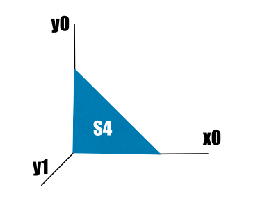
ITensor S1(x1,prime(x0,2),y0);
ITensor S2(y1,x0,y0);
ITensor S3(x1,x0,prime(y0,2));
ITensor S4(y1,prime(x0,2),prime(y0,2));

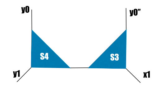
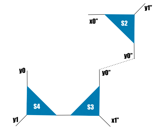
This pattern of tensors appears in a TRG calculation and this represents the final operation before updating the tensor for the next renormalization group step. In order to get a better idea of what these tensors look like, we should draw a picture:

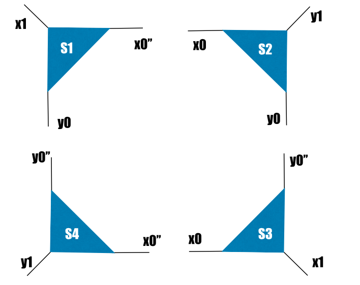
Right now, that's not what we want. If we contracted all the tensors (S1*S2*S3*S4), then we'd get a scalar. We want the diagrams to contract just as they are drawn: horizontal lines with horizontal lines, vertical lines with vertical lines. We also want some extra double primes on some of the level 1 indices (x1, y1). The tensors come out of the program this way and are a necessity in the TRG algorithm. We must manipulate the primes to get the correct contraction:

For educational purposes, let's prime one index:

prime(S1,y0);

and then unprime it

prime(S1,y0,-1);

This returns us to the original diagram.

Now we get serious. Let's remove all primes from S4:

A *= noprime(S4);//or mapprime(S4,2,0)

This is a promising step considering the contractions we eventually want. We then contract with S3:

A *= S3;

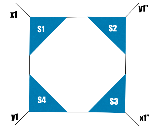
Now we prime twice the Xtype indices on the next contraction:

A = prime(A,Xtype,2);

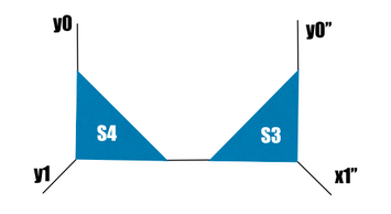
Let's prime S2 twice and contract it with A

A *= prime(S2,2);

The dotted line contracted on *. The last step is to contract S1 and this gives us the correct result.

A *= S1;

A more straightforward code would be:

auto l13 = commonIndex(S1,S3);//Obtains a common index from both S1 and S3
A = S1 * noprime(S4) * prime(S2,2) * prime(S3,l13,2);