Case Study: TRG Algorithm
The handful of techniques we have covered so far (ITensor contraction and SVD) are already enough to implement a powerful algorithm: the tensor renormalization group (TRG).
First proposed by Levin and Nave (cond-mat/0611687), TRG is a strategy for contracting a network of tensors connected in a two-dimensional lattice pattern by decimating the network in a heirarchical fashion. The term "renormalization group" refers to processes where less important information at small distance scales is repeatedly discarded until only the most important information remains.
The Problem
TRG can be used to compute certain large, non-trivial sums by exploiting the fact that they can be recast as the contraction of a lattice of small tensors.
A classic example of such a sum is the "partition function" @@Z@@ of the classical Ising model at temperature T, defined to be
where each Ising "spin" @@\sigma@@ is just a variable taking the values @@\sigma = +1, -1@@ and the energy @@E(\sigma_1,\sigma_2,\sigma_3,\ldots)@@ is the sum of products @@\sigma_i \sigma_j@@ of neighboring @@\sigma@@ variables. In the two-dimensional case described below, there is a "critical" temperature @@T_c=2.269\ldots@@ at which this Ising system develops an interesting hidden scale invariance.
One dimension
In one dimension, spins only have two neighbors since they are arranged along a chain. For a finite-size system of N Ising spins, the usual convention is to use periodic boundary conditions meaning that the Nth spin connects back to the first around a circle:
The classic "transfer matrix" trick for computing @@Z@@ goes as follows:
where @@\text{Tr}@@ means "trace" and the transfer matrix @@M@@ is a 2x2 matrix with elements
Pictorially, we can view @@\text{Tr}\left(M^N\right)@@ as a chain of tensor contractions around a circle:

With each 2-index tensor in the above diagram defined to equal the matrix M, it is an exact rewriting of the partition function @@Z@@ as a tensor network.
For this one-dimensional case, the trick to compute @@Z@@ is just to diagonalize @@M@@ . If @@M@@ has eigenvalues @@\lambda_1@@ and @@\lambda_2@@ , it follows that @@Z = \lambda_1^N + \lambda_2^N@@ by the basis invariance of the trace operation.
Two dimensions
Now let us consider the main problem of interest. For two dimensions, the energy function can be written as
where the notation @@\langle i j \rangle@@ means the sum only includes @@i,j@@ which are neighboring sites. It helps to visualize the system:
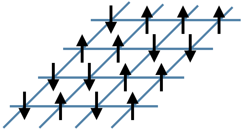
In the figure above, the black arrows are the Ising spins @@\sigma@@ and the blue lines represent the local energies @@\sigma_i \sigma_j@@ . The total energy @@E@@ of each configuration is the sum of all of these local energies.
Interestingly, it is again possible to rewrite the partition function sum @@Z@@ as a network of contracted tensors. Define the tensor @@A^{\sigma_u \sigma_r \sigma_d \sigma_l}@@ to be
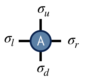
The interpretation of this tensor is that it computes the local energies between the four spins that live on its indices, and its value is the Boltzmann probability weight @@e^{-E/T}@@ associated with these energies. Note its similarity to the one-dimensional transfer matrix @@M@@ .
With @@A@@ thus defined, the partition function @@Z@@ for the two-dimensional Ising model can be found by contracting the following network of @@A@@ tensors:
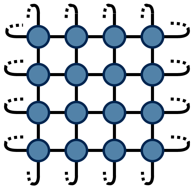
The above drawing is of a lattice of 32 Ising spins (recall that the spins live on the tensor indices). The indices at the edges of this square wrap around in a periodic fashion because the energy function was defined using periodic boundary conditions.
The TRG Algorithm
TRG is a strategy for computing the above 2d network, which is just equal to a single number @@Z@@ (since there are no uncontracted external indices). The TRG approach is to locally replace individual @@A@@ tensors with pairs of lower-rank tensors which guarantee the result of the contraction remains the same to a good approximation. These smaller tensors can then be recombined in a different way that results in a more sparse, yet equivalent network.
Referring to the original @@A@@ tensor as @@A_0@@ , the first "move" of TRG is to factorize the @@A_0@@ tensor in two different ways:

Both factorizations can be computed using the singular value decomposition (SVD). For example, to compute the first factorization, view @@A_0@@ as a matrix with a collective "row" index @@\sigma_l@@ and @@\sigma_u@@ and collective "column" index @@\sigma_d@@ and @@\sigma_r@@ . After performing an SVD of @@A_0@@ in this way, further factorize the singular value matrix @@S@@ as @@S = \sqrt{S} \sqrt{S}@@ and absorb each @@\sqrt{S}@@ factor into U and V to create the factors @@F_r@@ and @@F_l@@ . Pictorially:

Importantly, the SVD is only done approximately by retaining just the @@\chi@@ largest singular values and discarding the columns of U and V corresponding to the smaller singular values. This truncation is crucial for keeping the cost of the TRG algorithm under control.
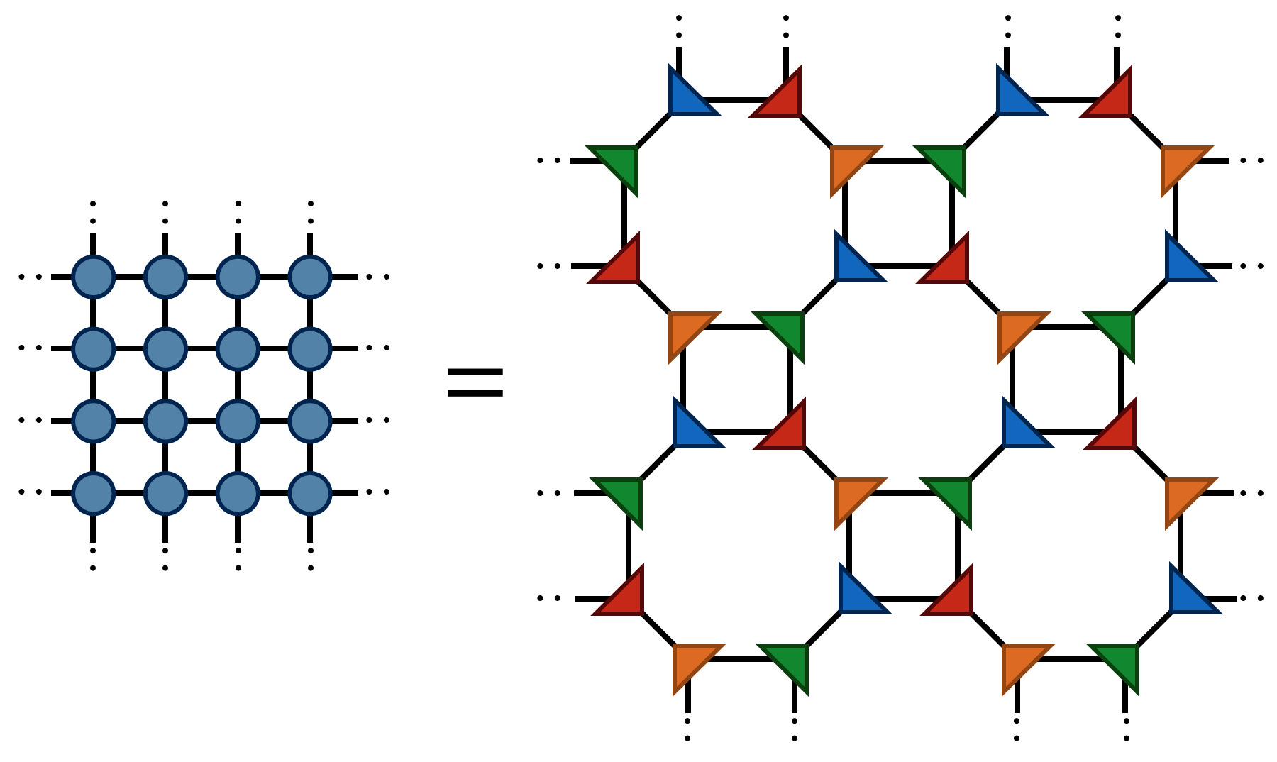
Making the above substitutions, either @@A_0=F_r F_l@@ or @@A_0=F_u F_d@@ on alternating lattice sites, transforms the original tensor network into the following network:
Finally by contracting the four F tensors in the following way
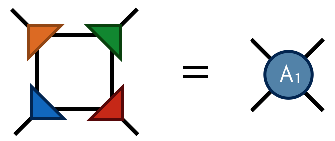
one obtains the tensor @@A_1@@ which has four indices just like @@A_0@@ . Contracting the @@A_1@@ tensors in a square-lattice pattern gives the same result (up to SVD truncation errors) as contracting the original @@A_0@@ tensors, only there are half as many @@A_1@@ tensors (each @@A_0@@ consists of two F's while each @@A_1@@ consists of four F's).
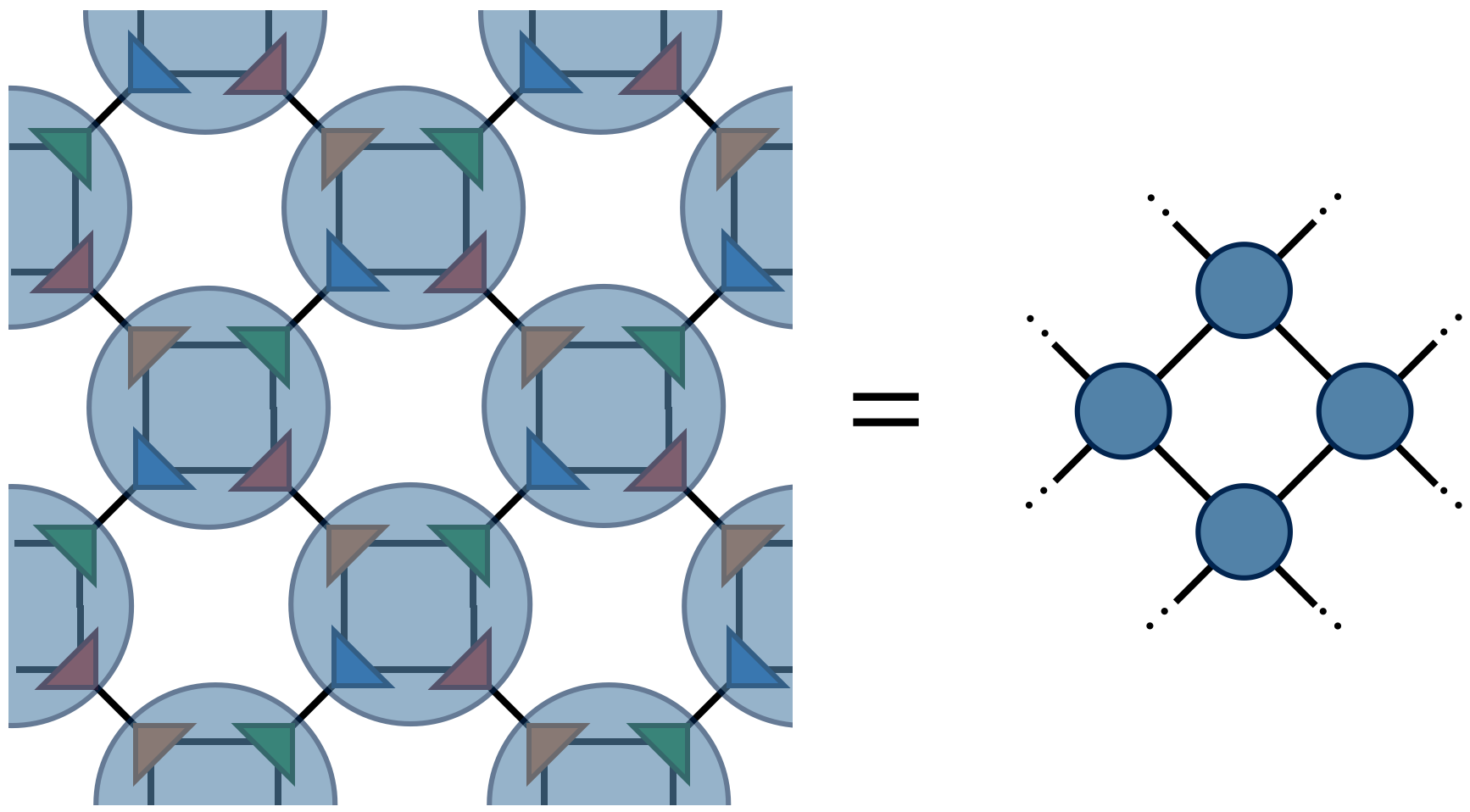
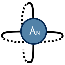
To compute @@Z@@ defined by contracting a square lattice of @@2^{1+N}@@ tensors, one repeats the above two steps (factor and recombine) N times until only a single tensor remains. Calling this final tensor @@A_N@@ , the result @@Z@@ of contracting the original network is equal to the following "double trace" of @@A_N@@ :
Implementing TRG in ITensor
Finally we are ready to implement the algorithm above using ITensor. At the end of this section we will arrive at a complete working code, but let's look at each piece step by step.
To get started, start with the following empty application:
#include "itensor/all.h"
#include "itensor/util/print_macro.h"

using namespace itensor;

int main()
{

//Our code will go here

return 0;
}
First define some basic parameters of the calculation, such as the temperature "T"; the maximum number of singular values "maxdim"; and the top-most scale we want to reach with TRG:
Real T = 3.0;
int maxdim = 20;
int topscale = 6;
Next define the indices which will go on the initial "A" tensor:
auto dim0 = 2;
auto s = Index(dim0,"scale=0");
auto l = addTags(s,"left");
auto r = addTags(s,"right");
auto u = addTags(s,"up");
auto d = addTags(s,"down");
Here it is good practice to save the index dimension @@dim0=2@@ into its own variable
to prevent "magic numbers" from appearing later in the code.
Copies of the same Index with different tags are considered to be distinct.
Therefore, we create the Index l by adding the tag "left", r by adding "right"
etc. to get distinct indices for the Boltzmann weight tensor A. Later as
the calculation runs, the "scale=0" tag will be replaced with "scale=1", "scale=2",
so that indices at different scales will be distinct too.
Now let's create the "A" tensor defining the partition function and set its values as discussed above:
auto A = ITensor(l,r,u,d);

auto Sig = [](int s) { return 1.-2.*(s-1); };

for(auto sl : range1(dim0))
for(auto sd : range1(dim0))
for(auto sr : range1(dim0))
for(auto su : range1(dim0))
    {
    auto E = Sig(sl)*Sig(sd)+Sig(sd)*Sig(sr)
            +Sig(sr)*Sig(su)+Sig(su)*Sig(sl);
    auto P = exp(-E/T);
    A.set(l=sl,d=sd,r=sr,u=su, P);
    }
The first line creates the "A" tensor with indices l,r,u,d and all elements set to zero.
The next line defines a "lambda" function bound to the variable name Sig which converts integers
1 and 2 into Ising spin values +1.0 and -1.0. To set the elements of A, we loop over integers
sl,sd,sr,su. The function range1(dim) returns an object that can be used in a for loop to
iterate over the integers 1,2,3,...,dim.
Finally we are ready to dive into the main TRG algorithm loop. To reach scale @@N@@ we need to do @@N-1@@ steps, so we will write a loop that does this number of steps:
for(auto scale : range(topscale))
    {
    printfln("\n---------- Scale %d -> %d  ----------",scale,1+scale);

    //...TRG algorithm code will go here...

    }
In contrast to the earlier range1 function which starts at 1, range(topscale) makes the for loop
run over 0,1,...,topscale-1.
Although on the first pass these are just the same indices we defined before, new indices will arise as A refers to tensors at higher scales.
Now it's time to decompose the current A tensor as discussed
in the previous section. First the A=Fl*Fr factorization:
auto [Fl,Fr] = factor(A,{r,d},{l,u},{"MaxDim=",maxdim,
                                     "Tags=","left,scale="+str(scale),
                                     "ShowEigs=",true});
When performing the factorization, we pass the tags we want the newly created Index
linking Fl to Fr to have ("left" and "scale=n").
The argument "MaxDim" puts a limit on how many singular values are kept in the SVD.
Setting "ShowEigs" to true shows helpful information about the truncation of singular values
(actually the squares of the singular values which are called "density matrix eigenvalues").
We can write very similar code to do the A=Fu*Fd factorization:
// Get the upper-right and lower-left tensors
auto [Fu,Fd] = factor(A,{l,d},{u,r},{"MaxDim=",maxdim,
                                     "Tags=","up,scale="+str(scale),
                                     "ShowEigs=",true});
Before contracting the F tensors back together to form the tensor definining the next scale, we need to make their shared indices distinct:
auto l_new = commonIndex(Fl,Fr);
auto r_new = replaceTags(l_new,"left","right");
Fr *= delta(l_new,r_new);

auto u_new = commonIndex(Fu,Fd);
auto d_new = replaceTags(u_new,"up","down");
Fd *= delta(u_new,d_new);
In the first line above, we grab the index connecting the Fl and Fr factor tensors.
Then we create an Index r_new which is like l_new but has
the tag "right" instead of "left", so that it will no longer be automatically contracted with l_new,
and similarly for u_new and d_new.
Having created these two new indices, we use a delta ITensor to replace l_new with
r_new on the ITensor Fr, and similar for Fd.
For the last step of the TRG algorithm we combine the factors of the A tensor at the current scale to create a "renormalized" A tensor at the next scale:
Fl *= delta(r,l);
Fu *= delta(d,u);
Fr *= delta(l,r);
Fd *= delta(u,d);

A = Fl * Fu * Fr * Fd;
The delta ITensors here are used to replace one Index by another, for example
the line Fl *= delta(r,l) replaces the r Index of Fl with the Index l.
Try drawing the tensor diagram showing the contraction
of the F tensors to convince yourself that the indexing works out correctly.
Before the next iteration begins, we update the variables l,r,u,d to ensure they are available for the next step:
l = l_new;
r = r_new;
u = u_new;
d = d_new;
To obtain @@Z@@ from the tensor at a given scale, all we have to do is trace the l and r indices with each other and trace the u and dindices with each other, which results in a scalar tensor whose value is @@Z@@ :

In ITensor, you can compute a trace by again using a delta ITensor
A delta tensor has only diagonal elements, all equal to 1.0.
Pictorially, you can view the delta tensors as the dashed lines in the above diagram.
Here is how the tracing of A works in our sample code:
Real TrA = elt(A*delta(l,r)*delta(u,d));
With this trace computed, we can normalize A at each step (A /= TrA) to
prevent the algorithm from encountering excessively large numbers
and we can update the partition function per site z:
z *= pow(TrA,1./pow(2,1+scale));
An interesting quantity to compute is @@\ln(Z)/N_s = \ln(z)@@ where @@N_s = 2^{1+N}@@
is the number of sites "contained" in the top tensor at scale @@N@@ .
With the conventions for the probability weights we have chosen, we can check
@@\ln(Z)/N_s@@ against the following exact result (for an infinite-sized system):
where the constant @@k=1/\sinh(2\beta)^2@@ and recall @@\beta=1/T@@ .
Click the link just below to view a complete, working sample code you can compile yourself. Compare the value of
@@\ln(Z)/N_s@@ you get to the exact result. How does adjusting maxdim and topscale affect your result?
#include "itensor/all.h"
#include "itensor/util/print_macro.h"
using namespace itensor;

int main()
{
Real T = 3.0;
int maxdim = 20;
int topscale = 8;

auto dim0 = 2;

// Define an initial Index making up
// the Ising partition function
auto s = Index(dim0,"scale=0");

// Define the indices of the scale-0
// Boltzmann weight tensor "A"
auto l = addTags(s,"left");
auto r = addTags(s,"right");
auto u = addTags(s,"up");
auto d = addTags(s,"down");

auto A = ITensor(l,r,u,d);

// Fill the A tensor with correct Boltzmann weights:
auto Sig = [](int s) { return 1.-2.*(s-1); };
for(auto sl : range1(dim0))
for(auto sd : range1(dim0))
for(auto sr : range1(dim0))
for(auto su : range1(dim0))
    {
    auto E = Sig(sl)*Sig(sd)+Sig(sd)*Sig(sr)
            +Sig(sr)*Sig(su)+Sig(su)*Sig(sl);
    auto P = exp(-E/T);
    A.set(l(sl),r(sr),u(su),d(sd),P);
    }

// Keep track of partition function per site, z = Z^(1/N)
Real z = 1.0;

for(auto scale : range1(topscale))
    {
    printfln("\n---------- Scale %d -> %d  ----------",scale-1,scale);

    // Get the upper-left and lower-right tensors
    auto [Fl,Fr] = factor(A,{r,d},{l,u},{"MaxDim=",maxdim,
                                         "Tags=","left,scale="+str(scale),
                                         "ShowEigs=",true});

    // Grab the new left Index
    auto l_new = commonIndex(Fl,Fr);

    // Get the upper-right and lower-left tensors
    auto [Fu,Fd] = factor(A,{l,d},{u,r},{"MaxDim=",maxdim,
                                         "Tags=","up,scale="+str(scale),
                                         "ShowEigs=",true});

    // Grab the new up Index
    auto u_new = commonIndex(Fu,Fd);

    // Make the new index of Fl distinct
    // from the new index of Fr by changing
    // the tag from "left" to "right"
    auto r_new = replaceTags(l_new,"left","right");
    Fr *= delta(l_new,r_new);

    // Make the new index of Fd distinct
    // from the new index of Fu by changing the tag
    // from "up" to "down"
    auto d_new = replaceTags(u_new,"up","down");
    Fd *= delta(u_new,d_new);

    Fl *= delta(r,l);
    Fu *= delta(d,u);
    Fr *= delta(l,r);
    Fd *= delta(u,d);
    A = Fl * Fu * Fr * Fd;

    Print(A);

    // Update the indices
    l = l_new;
    r = r_new;
    u = u_new;
    d = d_new;

    // Normalize the current tensor and keep track of
    // the total normalization
    Real TrA = elt(A*delta(l,r)*delta(u,d));
    A /= TrA;
    z *= pow(TrA,1./pow(2,1+scale));

    }

printfln("log(Z)/N = %.12f",log(z));


return 0;
}
 Download the full example code
Next Steps for You to Try
Modify the sample application to read in parameters from a file, using the ITensor input parameter system.
Following the details in the appendix of the "Tensor Network Renormalization" paper arxiv:1412.0732, for the critical temperature @@T_c=2/\ln(1+\sqrt{2})@@ trace the top-scale "A" tensor in the x direction, then diagonalize the resulting matrix to obtain the leading scaling dimensions of the critical 2 dimensional Ising model.
Following the paper arxiv:0903.1069, include an "impurity tensor" which measures the magnetization of a single Ising spin, and compare your results at various temperatures to the exact solution.
References
The original paper on TRG:
Levin and Nave, "Tensor Renormalization Group Approach to Two-Dimensional Classical Lattice Models", PRL 99, 120601 (2007) cond-mat/0611687
Paper on TRG with very useful figures (particularly Fig. 5):
Gu, Levin, and Wen, "Tensor-entanglement renormalization group approach as a unified method for symmetry breaking and topological phase transitions" PRB 78, 205116 (2008) arxiv:0806.3509
TNR is an extension of TRG which qualitatively improves TRG's fixed-point behavior and can be used to generate MERA tensor networks:
Evenbly and Vidal, "Tensor Network Renormalization" PRL 115, 180405 (2015) arxiv:1412.0732

